Publisher

2.1 Author name Fennica

MARC: 100a

Author’s name section’s summary tables offer insights into the dataset’s integrity, illustrating the accepted and discarded author names. An examination of missing values in the original dataset provides transparency regarding data completeness. The inclusion of information on name variants and pseudonyms enriches the analysis, addressing nuances in authorship representation. This comprehensive approach ensures a thorough understanding of the dataset’s composition and the intricacies associated with author identification.

2.1.1 Complete Dataset Overview

2.1.1.1 Authors

  • 195920 unique authors These final names capture all name variants from the custom author synonyme table, and exclude known pseudonymes (see below). If multiple names for the same author are still observed on this list, they should be added on the author synonyme table.

  • 0 documents have unambiguous author information (NaN%).

  • Author name conversions Non-trivial conversions from the original raw data to final names.

#Author’s name (100a) - Top 10

2.1.1.2 Auxiliary files

2.1.2 Subset Analysis: 1809-1917

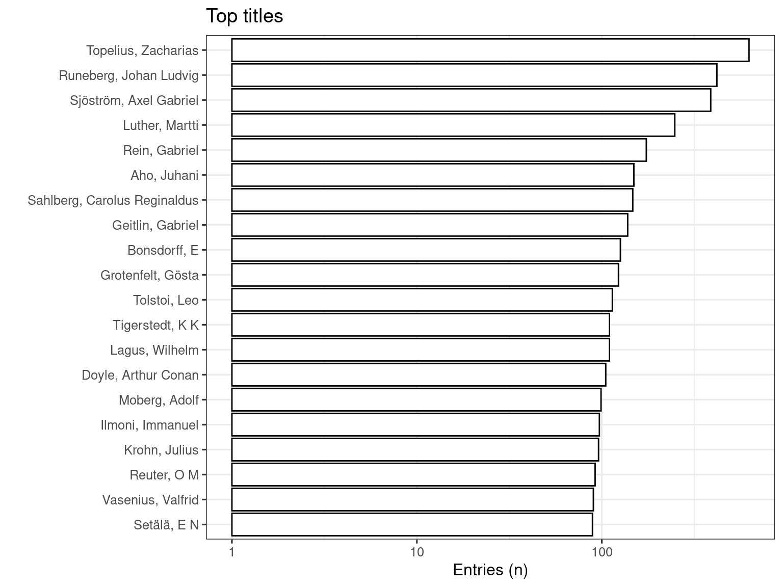
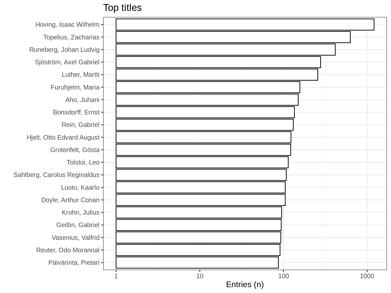
Top-20 titles and their title counts for period 1809-1917.

The accompanying plot visually underscores the prominence of these authors, emphasizing the metric of the number of unique titles published by each author.
3 Author’s name after integration

4 Author’s Name after Kanto integration

5 1809-1917 all names

#| include = FALSE
source("init.R")
source("publication_time.R")
source("gender.R")
field <- "gender_primary"

5.1 Author’s Gender

Gender information is not originally included in Fennica. We enriched the data by linking author names with gender information from various sources, including the HENKO project, the Genderize dataset, manual curation and search, and additional records provided by the National Library of Finland. The full list of names and genders can be found here.

In total N = r nrow(df) records. After enrichment in total there are records r sum(!is.na(df[[field]])) / (r round(100*mean(!is.na(df[[field]])), 1)%) with assigned gender. There are r sum(df[[field]] == "female", na.rm = TRUE) (r round(100*mean(df[[field]] == "female", na.rm = TRUE), 1)%) female names, r sum(df[[field]] == "male", na.rm = TRUE) (r round(100*mean(df[[field]] == "male", na.rm = TRUE), 1)%) male names and r sum(df[[field]] == "unisex", na.rm = TRUE) (r round(100*mean(df[[field]] == "unisex", na.rm = TRUE), 1)%) unisex names.

5.1.1 Gender over Time (1600-2000)

#| label = "summary_gender",
#| echo = FALSE,
#| warning = FALSE,
# Join publication_decade from df_pubtime to df by melinda_id
df$publication_decade <- df_pubtime$publication_decade[match(df$melinda_id, df_pubtime$melinda_id)]

# Filter your data to only include those genres
df_selected <- df%>%
  filter(!is.na(publication_decade), 
         !is.na(gender_primary),
         publication_decade <= 2000)

# Summarize counts by decade and genre
df_summary <- df_selected %>%
  group_by(publication_decade, gender_primary) %>%
  summarise(n = n(), .groups = "drop")

ggplot(df_summary, aes(x = publication_decade,y = n, fill = gender_primary)) +
  geom_col(position = "stack", width = 8) +  # width makes bars a bit narrower
  labs(x = "Publication Decade", y = "Gender count", fill = "Gender") +
  scale_fill_brewer(palette = "Set2") +
  scale_x_continuous(limits = c(1600, 2000),breaks = seq(1600, 2000, by = 50)) +
  theme_minimal()

5.1.2 Gender over Time (1809-1917)

#| label = "summary_gender19",
#| echo = FALSE,
#| warning = FALSE,
# Join publication_decade from df_pubtime to df by melinda_id
df_19$publication_decade <- df_pubtime19$publication_decade[match(df_19$melinda_id, df_pubtime19$melinda_id)]

# Filter your data to only include those genres
df_selected <- df_19 %>%
  filter(
    !is.na(publication_decade),
    !is.na(gender_primary),
    publication_decade >= 1800 & publication_decade <= 1920
  )

# Summarize counts by decade and genre
df_summary <- df_selected %>%
  group_by(publication_decade, gender_primary) %>%
  summarise(n = n(), .groups = "drop")

ggplot(df_summary, aes(x = publication_decade,y = n, fill = gender_primary)) +
  geom_col(position = "stack", width = 8) +  # width makes bars a bit narrower
  labs(x = "Publication Decade", y = "Gender count", fill = "Gender") +
  scale_fill_brewer(palette = "Set2") +
  scale_x_continuous(limits = c(1800, 1920),breaks = seq(1800, 1920, by = 50)) +
  theme_minimal()
#| include = FALSE
source("init.R")
source("publication_time.R")
source("author_profession.R")

5.2 Author’s profession

Auhtor profession in fennica is depicted in 700,e field. We enrich it with information from Kanto. In total N = r nrow(df) records. Before enrichment 700,e has r sum(is.na(df[[field]])) / (r round(100*mean(is.na(df[[field]])), 1)%) missing values. After enrichment in total there are records r sum(!is.na(df[[field]])) / (r round(100*mean(!is.na(df_19[[field]])), 1)%) with assigned profession. There are r length(unique(na.omit(df[[field]]))) professions.

#| label = "summaryproffesion",
#| echo = FALSE,
#| results = "asis"
x <- top(df, "author_profession")
tab <- cbind(names(x), unname(x), round(100 * unname(x/nrow(df)), 1))
colnames(tab) <- c("Profession", "Entries (n)", "Fraction (%)")
kable(head(tab, 15))
#| label = "source-index",
#| include = FALSE
source("init.R")
source("publisher.R")

MARC: 260b

5.3 Complete Dataset Overview

5.4 Subset Analysis: 1809-1917

  • r length(unique(df_19$publisher)) unique publishers

  • r sum(!is.na(df_19$publisher)) documents have unambiguous publisher information (r round(100*mean(!is.na(df_19$publisher)), 1)%). This includes documents identified as self-published; the author name is used as the publisher in those cases (if known).

  • Discarded publisher entries

The r ntop most common publishers from 1809 to 1917 are shown with the number of documents.

#| label = "summarypublisher2",
#| echo = FALSE,
#| message = FALSE,
#| warning = FALSE,
#| fig.width = 12,
#| fig.height = 9
p <- top_plot(df_19, "publisher", ntop)
p <- p + ggtitle(paste("Top publishers"))
p <- p + scale_y_log10()
p <- p + ylab("Documents")
print(p)